Tagged with system dynamics

St. Matthew Island. On reindeer and lichen

Today is all about reindeer. I stumbled upon this comic the other day and was delighted. I had seen it some time ago and thought it to be very neatly relevant to system dynamics. And had lost the link. Anyway, here is the link, go read it or the rest will make no damn sense.

Done?

OK, I’ll give you a minute.

Done? Good.

My interest in this is twofold. Firstly, this comic is a direct reflection of what World Dynamics is all about and secondly I’d very much like to put some numbers behind the story and the ecosystem structure should be for something like this to happen. Typically a case like this is used to illustrate a point of over-compensation: herd growth does not stop when the food runs out (as there are a number of calves underway) so the population grows beyond what the ecosystem can sustain.

I built a model. Actually I built several. And I did not get the behavior depicted in the diagram. The thing is that there are no right angles in nature. All the reindeer just didn’t eat happily to their hearts content one day and were utterly out of food the next. Also, lichen reproduces so slowly that we can assume the island can not sustain a single reindeer on just lichen growth alone. Therefore, lichen will run totally out at some point regardless of how the herd behaves (the consumption exceeds growth) and therefore the overcompensation concept does not apply: the model starts off in a point where it is already beyond the limit.

I inevitably ended up with a nice bell curve: the population grows to a point where the lichen starts having an effect on both fertility and longevity and its a nice steady decline to zero from there. as the food gets gradually scarcer. The important conclusion is that the result is symmetrical: exponential growth is followed by exponential decline.

Here’s the thing. Maybe what the people saw was _not_ the peak but rather the decline? If we assume that the island at some point had not 6 bot about 12 thousand reindeer, we can easily find a normal distribution curve that very closely fits the observation points. Which, of course, means that there was no dramatic cliff the population stumbled over. Don’t get me wrong, halving the population in a couple of years is dramatic as well but the diagram in the cartoon seems off. I’ll ponder over it for a while and see if I come up with an alternative solution but that’s that for the moment

Oh, and a notice: the next two weeks are going to be the peak of my thesis-writing so I might not get around to come up with stuff to post here – it takes considerable time and while superinteresting, I need to get the thesis done. Whatever I do, you should be enjoying system dynamics in action!

Tagged , , , ,

On traffic

Oh dear, some horrible things happened around here with the gunman in the movies. For a second there I thought hey, this is a simple feedback loop between guns in the hands of criminals and guns in the hands of citizens, let’s make a post. Then I realized the magnitude of wrongness of me doing that. I also realized that the system is actually not that simple at all. Thus, we will continue with our regular programming delayed by a technical glitch and come back to the guns thing at a later time if at all.


Today we talk about traffic. Not least because this week professor Jay Forrester gave his lecture to the System Dynamics class. He is, of course, the grand old man of urban studies and last year at the same class he said something really interesting (am quoting from memory) about the topic: “Whenever you decide to make something better, you are just pushing bottlenecks around. You need to decide, what you are willing to make _worse_ in order to achieve a lasting result”

I have lately made the mistake of following up on Estonian media and, based on the coverage, one of the most pressing issues there is that the city of Tallinn has overnight and without much warning halved the throughput of certain key streets.

While we speak, the Euro is falling, US is in the middle of a presidential debate, the Arab world is in flames, we are on a verge of a paradigm shift in science, Japan is making a huge change in their energy policy possibly triggering a global shift and all of this is surrounded by general climate change and running out of oil business.

Oh, well. We probably all deserve our parents, children, rulers and journalists.

Anyway, that piece of news seemed to match perfectly the words of Jay Forrester and thus todays topic.

What the quote above means is that tweaking system values will just prompt more tweaking. Making a road wider will encourage more people to drive on it necessitating expansion of source and sink roads which have source and sink roads of their own. Thus, what professor Forrester says is that in order for that cycle to stop, one must make a conscious decision _not_ to improve certain things. Yes, traffic is horrible but instead of adding more roads, what else can we do? How can we change the structure of the system rather than tweaking and re-tweaking certain values that will only result our target variable stabilize at a (hopefully more beneficial) level?

This brings us back to Tallinn. From one hand it might seem that the change is in the right direction: somebody has decided to make the lives of drivers worse in order to stop pushing the bottlenecks around.

Applause!

Or maybe not. You see, what Jay Forrester definitely did not mean was that _any_ action resulting in somebody being worse off is beneficial for the system. Only careful analysis can reveal what change can overcome the policy resistance of a given system.

The following is based on public statements about the future of public transport in Tallinn as reflected by media. It would certainly be better to base them on some strategy or vision document but alas, there is none. At least to my knowledge and not in public domain. There was a draft available on the internet for comments last summer but that’s it.

Uhoh.

Let’s see, then. When driving restrictions are applied, two things happen. Firstly, amount of people driving will go down simply because it is inconvenient but also, the _desire_ to go downtown will diminish after a while. I’ll go to the local shop instead of driving. Let’s lease our new office space somewhere with good access rather than downtown. That sort of thing. When willingness to drive downtown diminishes, amount of people driving certainly goes down but so will the number of people taking the bus: if the need and desire are gone, there is no point in standing in the bus stop, is there?

It has been publicly stated that the money acquired from making the lives of drivers harder (this includes high parking fees, among other things) will be used to fund adding capacity to public transport. Therefore, the less people drive, the less money there is to maintain some headroom in terms of capacity. The less headroom we have the higher the chance that the person taking the bus does not want to repeat the experience and prefers not to the next time. And, of course, investment in the road network drives up the amount of people who actually drive.

Simple, isn’t it? Before I forget, many of these causal relationships have delays. Offices do not get moved and shops built overnight, investments take time to show results. It takes time for people to realize they don’t actually want to spend 2 hours each day in traffic.

Here’s a diagram of the system I described.
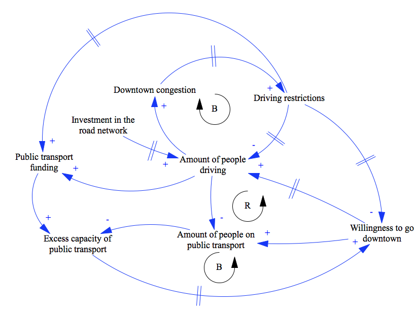
Now, tell me, what changes in what variables and when will result in sudden and rapid increase in driving restrictions that occur simultaneously to a massive investment to road infrastructure at city boundary?

Nope, I have no idea either. From the structural standpoint, the system is a reinforcing loop surrounded by numerous balancing loops. Since several of them involve delays, it is very hard to tell whether the system would stabilize and when. It seems though that in any case, a reinforcing loop driving down the willingness of people to go downtown gets triggered. The danger with these things is, of course, that when they _don’t_ stabilize or stabilize at a lower level than desired, downtown will be deserted and left only to tourists (if any) as the need to go there diminishes. The citizens not being in downtown kind of defies the point of making that downtown a more pleasurable place, doesn’t it?

Surprisingly, the city of Tallinn has actually done some things to break the loops described. For example, the public transport system has operated on non-economic principles for years and years. The city just pays for any losses and there is no incentive to make a profit. This makes the system simpler and removes a couple of fast-moving economic feedback loops. For this particular campaign, however, taxation on drivers was specifically announced as a funding source for public transportation without much further explanation.

The system is an interesting one and had I some numbers to go on, would be fun to simulate. But I think I have made my point here. Urban transportation is a problem of high dynamic complexity. When the system described above was to be cast into differential equations, there would unlikely to be an analytical solution. How many of you can more or less correctly guess a solution to a Nth order system of partial differential equation? Without actually having the equations in front of you? Do it numerically? Right.

It is thus imperative that decisions that could easily result in rather severe consequences to the city are based on some science or are at least synchronized amongst each other (did I mention it? There is a multi hundred million euro development project underway to radically increase the capacity of a certain traffic hotspot in Tallinn) using some sort of common roadmap.

I hope this excursion into local municipal politics still provided some thoughts on system dynamics in general and hope you’ll enjoy some of it in action over a safe weekend!

Tagged , , , ,

On changes

H’llo, here we go again!

Last time I promised I’d have some neat numbers for you but first, let’s talk about changes. Not like changing your hair color or favorite brand of root beer but changes in projects. Everybody knows they can be dangerous and implementing a proper change management procedure is one of the first things project managers are taught. And yet, change management can be a downfall of even the most well-managed projects. For instance, the Ingalls shipbuilding case I have referred to earlier.

Footnote: My favorite case ever on project management is also about changes. The Vasa was to be the pride of the Swedish navy in 1628 but sank on its maiden voyage in front of thousands of spectators. The reason? The king demanded addition of another gun deck dangerously altering the center of gravity of the ship. The jest of the story? The ship contained wooden statues of the project managers and those are now on display in the Vasa Museum in Stockholm. Get change management wrong and chances are 400 years later people will laugh and point fingers at your face.

Why is this? Mainly because of the difficulties of assessing impact. While direct costs involved in ripping out work already done and adding more work can be estimated with relative ease, the secondary effects are hard to estimate. Are we sure ripping out stuff wont’ disturb anything else? How many mistakes are we going to make while doing the additional work, how many mistakes will slip through tests and how many mistakes will the fixes contain? As the case referred to earlier illustrates, this is a non-trivial question.

“Yes”, you say, ” this is why good project managers add a wee bit of buffer and it is going to be fine in the end”. Really? How much buffer should you add, pray? Simulation to the rescue!

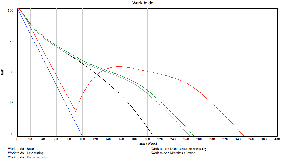
What I did was to add 10 tasks worth of work to a project of 100 tasks. 10% growth. I did this in a couple of ways. Firstly, I made the new stuff appear over 10 days early in the project, then the same late in the project and then added 10 tasks as a constant trickle spread over the entire project. Here are the results:

What’s that butt-ugly red thing, you ask? Oh, that’s something special we already had a brush with an an earlier post. You see, sometimes projects are set up so that the customer does not accept or test anything before there is something to really show off and that is late in the project. Of course, this means that the customer can not come up with any changes before that delivery happens and of course no mistakes are discovered either. The thing I like most about the red bar is how the amount of work to be done doubles after the testing starts. For the project manager this means that there is no way to even assess the quality of their work and thus there is no way to tell, if you are meeting the schedule and budget or not and the actual project duration is FOUR TIMES longer than projected based on initial progress…

I realize the graph is a bit of a mess so here’s a helpful table:

Tasks done Percentage added to base Multiplier to work added
Base case 336.42 0.00% 0.00
New work added early 357.89 6.38% 2.15
New work added late 369.82 9.93% 3.34
Late acceptance 429.077 27.54% 9.27
Trickle 361.369 7.42% 2.49

I chose not to review the deadlines as we are trying to asses the cost and not deadline impact of a change. The amount of work actually done is much more telling.

The first column shows the number of tasks actually done at the end of the project. For base case (the productivity and failure parameters are similar to the ones used in the previous post), this is 336.42. This should not come as a surprise to you, dear reader, but stop for a moment to digest this. In an almost ideal case the project takes 3.36 times more effort than would be expected.

The second column shows how many percentages the scenario adds to the tasks done in base case and the third one shows by how much these ten additional tasks got multiplied in the end.

Not very surprisingly, the best case scenario is to get the changes done with early on in the project. This is often not feasible as the customer simply will not know what the hell they want and so, realistically, trickle is the practical choice. By the way, this is where agile projects save tons of effort. Adding new work late is much worse, 10 new tasks become 33.4.

Now, close your eyes and imagine explaining your customer that a change that adds $1000 worth of effort to the project should be billed as $3340.

Done? At what price did you settle? Well, every dollar lost represents a direct loss to your company as the costs will be incurred regardless of whether or not the customer believes in this or not. To put this into perspective, 11.93 tasks worth of work can be saved if the customer comes up with a change earlier. Esteemed customer, this is the cost of you not telling the contractor about changing your mind early enough.

By far the worst case is the late testing. The effort goes up by almost an order of magnitude! That’s really not cool. Who does that sort of thing, anyway? Come to think of it, anybody who does classical one-stage waterfall which is an alarming percentage of large government contracts and a lot of EU-funded stuff. Scary. Nobody wins, you see. Even if the contractor, through some miracle of salesmanship combined with accounting magic, manages to hide the huge additional cost somewhere in the budget, they are unlikely to be able to hide the cost and the margin so the contractors overall margin on the project goes way down while the costs for the customer go up. They could choose to change the process instead and split the 2/3 of the savings between themselves… Wouldn’t it be lovely?

Let’s hang on to that thought until next week. Meanwhile, do observer System Dynamics in Action!

Tagged , , ,

Why are projects late?

It’s this time of the week again, time for another episode of (drumroll) SD Action!

Last time I introduced a basic project management model, this time let’s look at what this baby can do.

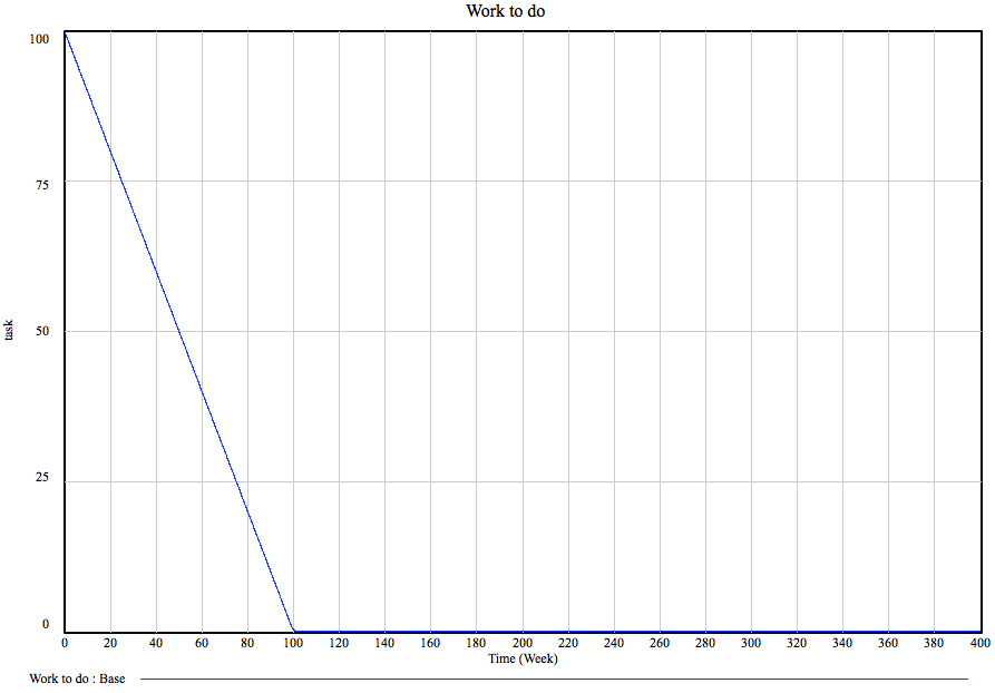
Let our base project be a project with 100 tasks. The team size is 200 people, each of whom can accomplish 0.005 tasks per week, this leads to… Oh, I don’t know. Here’s a graph:

Yup, the amount of work to be done (see the previous post for the model framework) goes down at a steady rate and the project is done by the one hundredth week. Nice. I can hear the more experienced project managers go “yeah, right!” Nothing ever goes as smoothly, people make mistakes! You’re supposed to add buffers and such, 30% is the standard practice.

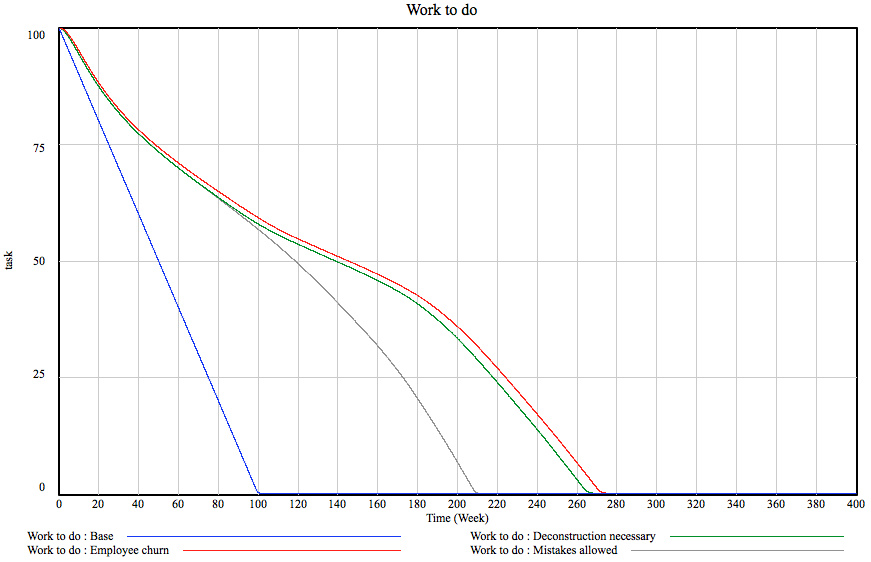
Hm, let’s see what happens if we allow people to make mistakes. On the model, this amounts to there being 20% of chance of a task to have the need to be re-done and the rework generation and discovery flows kicking in. Given the one fifth chance of a mistake, how much should we add to the project duration? 20%, right? Not exactly. You see, you might make mistakes on the bug fixes as well… You guessed it, here’s a graph:


What kind of sorcery is this? The project duration did not grow by 20% and not even 30%. It grew by 110%! Blimey, we just missed our deadline.

Oh well. Sure. Mistakes happen. But what if the mistakes are costly, generating more work to remove the previously done stuff? Remember the example of having to chip out old concrete before pouring new. Here we go:

Yes, this added another 55 weeks to the project. This is one year. By allowing mistakes to cause additional work. Of course, the relationships are more subtle but they are way too geeky to explain here. The deconstruction rate depends on how much of the project is done: it is 0 for about 50% and grows to 1 (in the later phase, as much of effort goes into deconstruction as into rework) as the project progresses. These assumptions are probably different in your field but in my world, one year got added to the project by making a fairly reasonable assumptions of mistakes costing effort.

As said earlier, the team size is 200 people. Given that at this point we are looking at a five-year project, it would be reasonable to assume that there is employee churn. Of course, the newcomers must learn the ropes before they can be productive and, in fact, the entire team starts out this way having about half the productivity. Let’s assume there is 10% employee churn annually, hiring is started immediately to replace the leavers (6 weeks to fill a position on average) and that it takes four weeks to get acquainted with the project.

This is actually not half bad, we loose only 5 weeks or so. It turns out that 10% churn in 200-person team is not a big deal. What is curious, though, that most of the lag is caused by the the fact that the team size actually goes down. How come? You see, given the parameters, the churn turns out to be faster than hiring. People leave until annual churn drops to the same level as hiring and stops there, the model stabilizes. In our case, this means there are 195 productive people, 3 people are constantly in incubation and 2 are just lost. This is where system dynamic modeling excels: solving this symbolically would have involved constructing and solving a system of differential equations but I just drew a couple of boxes and pressed a button.

How many of you have spotted a fatal flaw in the model? You did? Right! Give the gal a cookie!

Let’s give others a moment, shall we…

Yes, right. The thing is that the current model assumes testing starts immediately. The moment anybody writes a line of code or draws a line, it gets tested and, after a while, possible mistakes end up back at the work queue. Unfortunately, this is not how stuff happens in many cases.

Let’s take construction. Firstly, the architect dreams up a house. Then a bunch of engineers figure out the structure of the thing. Then people come and work on pipes, ventilation and drains. And finally somebody devises a loom of electric wires. And then people go and start building it only to discover that a ventilation duct must pass directly through a structural beam. And a cable ladder crosses a flight of chairs. At about chest height. Bummer. With the way construction is done in this country, I’m assured, there are very little means to discover such mistakes before construction actually begins. In our model, I’ve made it so that there is no rework discovery until about a third through the project, then everything proceeds normally. This is how it goes:

Sweet mother of baby Jesus! 80 weeks! Of course I’m overdoing things a bit. Some testing does happen earlier. True. But the current model does not account for any customer spec changes or for any risk materializing so, broadly speaking, the order of magnitude – about 30% – should be in the ballpark. What is worth, though, is this:

The graph shows the ratio of percentage of work actually done and the percentage of work believed to be done. For all other cases, it peaks pretty early on and starts declining nicely but for late testing, it remains very high until very late. For a project manager this means that they have no idea whatsoever how the project is progressing. Which is a Bad Thing ™.

Let’s recap. By adding only four simple aspects of project behavior, our project has grown 350% in the worst case and about 250% for sensible testing behavior. And we still have not talked about risks or awkward acceptance tests or multiple contractors or, or… Oh God.

See, this is why projects are late. Project managers are faced with dynamically complex systems that can go off on wild tangents for any reason and usually only have their gut to rely on. Of course, being under deadline pressure and lacking concrete evidence they give in and promise these 100 weeks or possibly 150. Well, they should go and simulate their project model and see what comes out the other end. In short, they should observe System Dynamics in Action!

Tagged , , , ,